Section 6: Linear Regression
Sam Frederick
Columbia University
3/28/23
Last Section
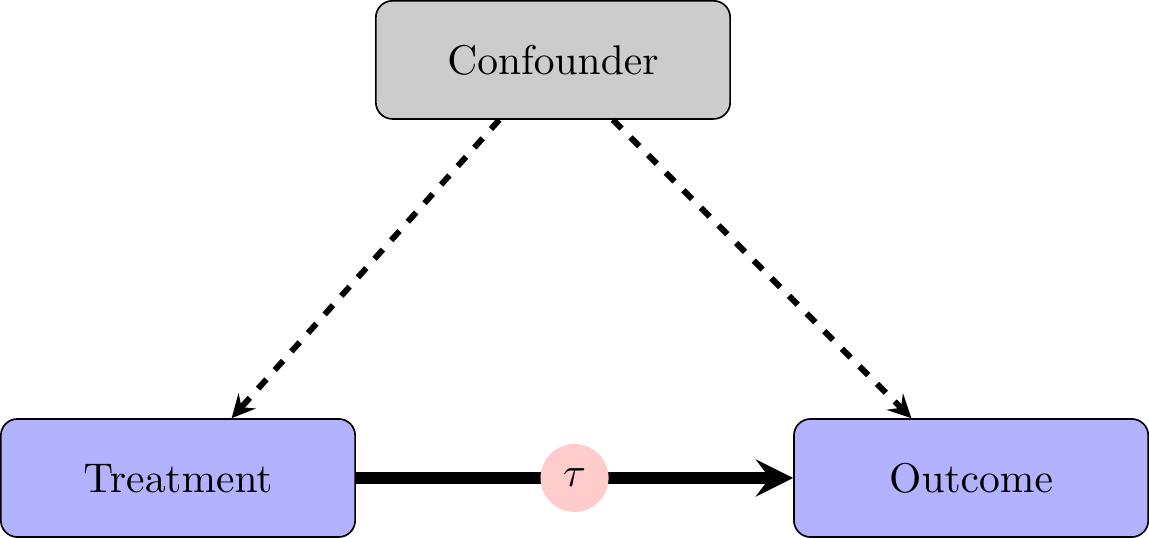
Confounding Variables
Randomized Experiments
Observational Data
- Can’t always randomly assign treatments of interest
- Governmental policies
- Individual characterstics
- Harmful occurrences/events (e.g., wars)
- How can we study the effects of these “treatments” without randomization?
- Regression
Regression
- Try to hold other variables constant
- Compare apples to apples (like units in “treatment” and “control” groups)
- Requirement for estimation of causal effects in observational studies:
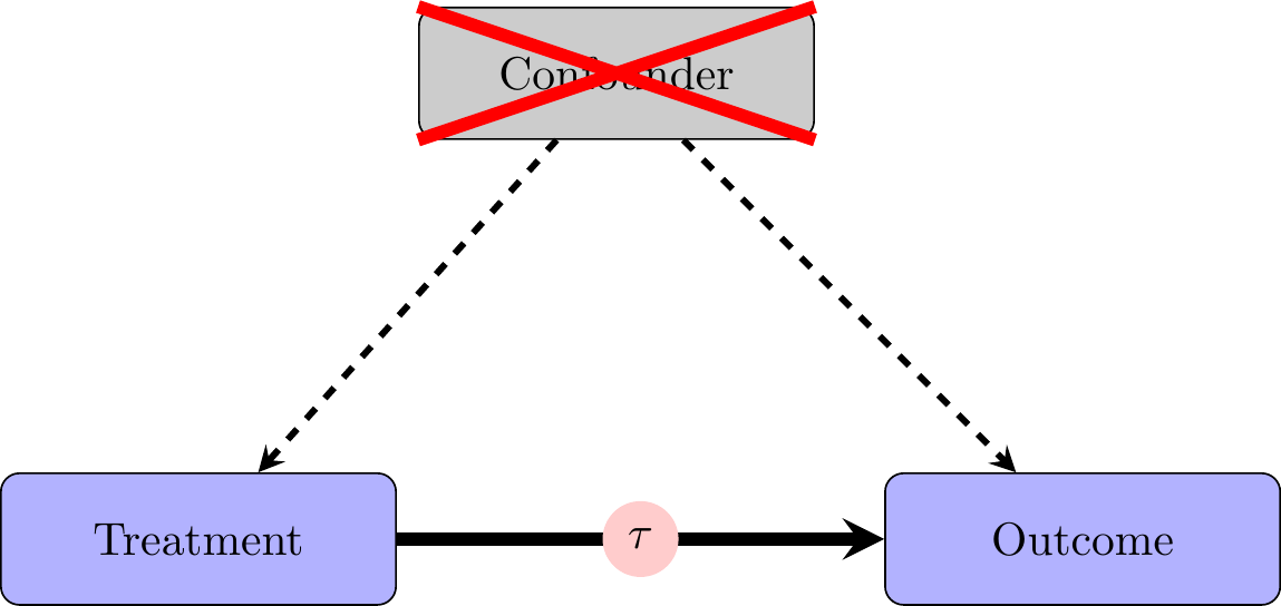
- No confounding variables
- “control” for all confounders/include them in the regression model
- No confounding variables
Confounding Variables
- Usually cannot be sure that there are no confounders
- That’s why experiments are ideal
- Estimates can be badly biased if there are unobserved confounding variables
- Known as omitted variable bias
Regression
- \(y = \alpha + \beta X + \varepsilon\)
- \(y\) is the dependent/outcome variable
- \(X\) is the independent/predictor variable
- \(\alpha\) is the y-intercept (the average value of y when other variables are 0)
- \(\beta\) is the slope or the coefficient estimate for X
- \(\varepsilon\) is variation in outcome “unexplained” by the model
Regression
- Start with
experiment.csv
- Simple experimental example
- True equation is \(y = 3 + 4*treatment + \varepsilon\)
- Remember \(y = \alpha + \beta X\)
Regression
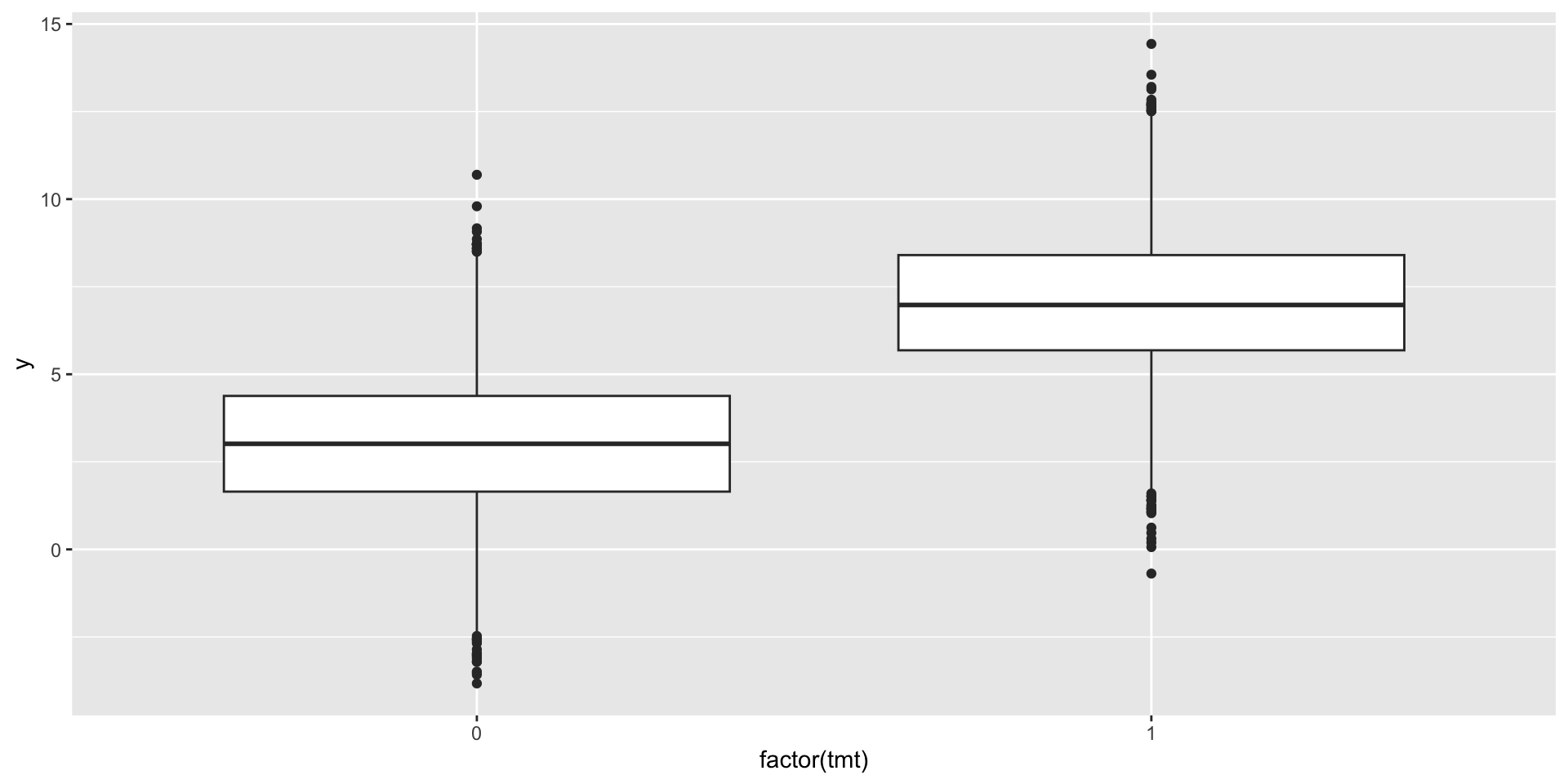
Regression
- In the past, we used a t-test/calculated the difference-in-means estimate by hand
[1] 3.991027
    Welch Two Sample t-test

data:  y by tmt
t = -99.58, df = 9991.4, p-value < 2.2e-16
alternative hypothesis: true difference in means between group 0 and group 1 is not equal to 0
95 percent confidence interval:
 -4.069589 -3.912465
sample estimates:
mean in group 0 mean in group 1
       3.008432        6.999459
Regression
We can accomplish this as well using regression
In R, run regressions using
lm()commandlm(y~x, data = dataname)
Regression
Regression
Call:
lm(formula = y ~ tmt, data = data1)

Residuals:
    Min      1Q  Median      3Q     Max
-7.6901 -1.3320 -0.0103  1.3873  7.6871

Coefficients:
            Estimate Std. Error t value Pr(>|t|)
(Intercept)  3.00843    0.02818  106.77   <2e-16 ***
tmt          3.99103    0.04008   99.58   <2e-16 ***
---
Signif. codes:  0 '***' 0.001 '**' 0.01 '*' 0.05 '.' 0.1 ' ' 1

Residual standard error: 2.004 on 9998 degrees of freedom
Multiple R-squared:  0.498, Adjusted R-squared:  0.4979
F-statistic:  9917 on 1 and 9998 DF,  p-value: < 2.2e-16
Regression
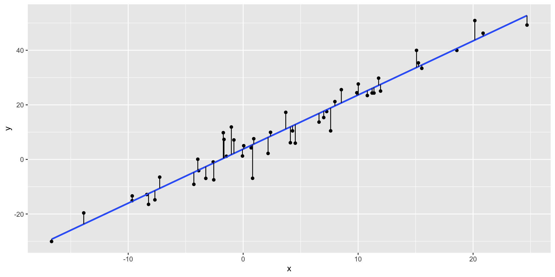
- What is regression doing?
- It is finding the line that minimizes the sum of squared residuals
- Sum of Squared Residuals:
- Residual: difference between prediction from regression and true outcome variable value
- \(SSR = \sum_{i=1}^n (\hat{y}_i - y_{i})^2\)
Regression
- Take a look at
regression_data.csv
- True equation: \(y = 3 + 2*x + \varepsilon\)
Regression
- Let’s make a scatterplot of the data
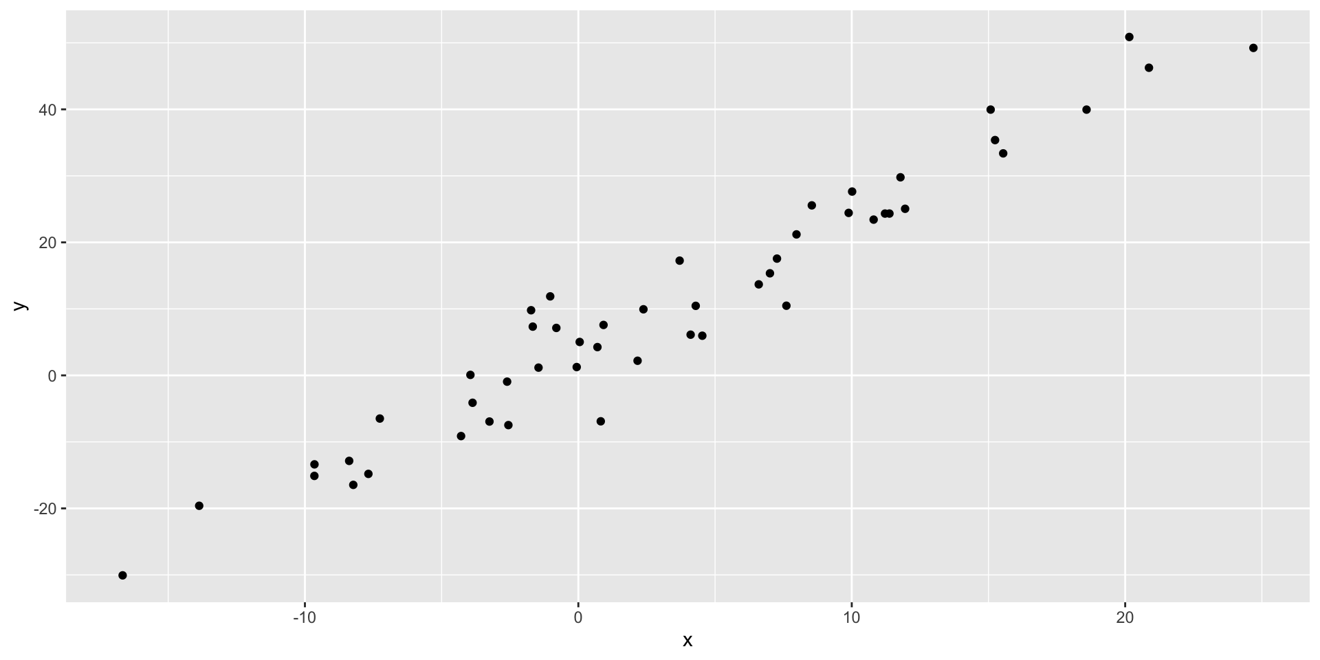
Regression
Regression
Call:
lm(formula = y ~ x, data = data2)

Residuals:
     Min       1Q   Median       3Q      Max
-12.3222  -2.4311  -0.1352   2.4702  10.1279

Coefficients:
            Estimate Std. Error t value Pr(>|t|)
(Intercept)  3.79069    0.68815   5.509  1.4e-06 ***
x            1.98246    0.07053  28.107  < 2e-16 ***
---
Signif. codes:  0 '***' 0.001 '**' 0.01 '*' 0.05 '.' 0.1 ' ' 1

Residual standard error: 4.571 on 48 degrees of freedom
Multiple R-squared:  0.9427,    Adjusted R-squared:  0.9415
F-statistic:   790 on 1 and 48 DF,  p-value: < 2.2e-16
Regression
Regression

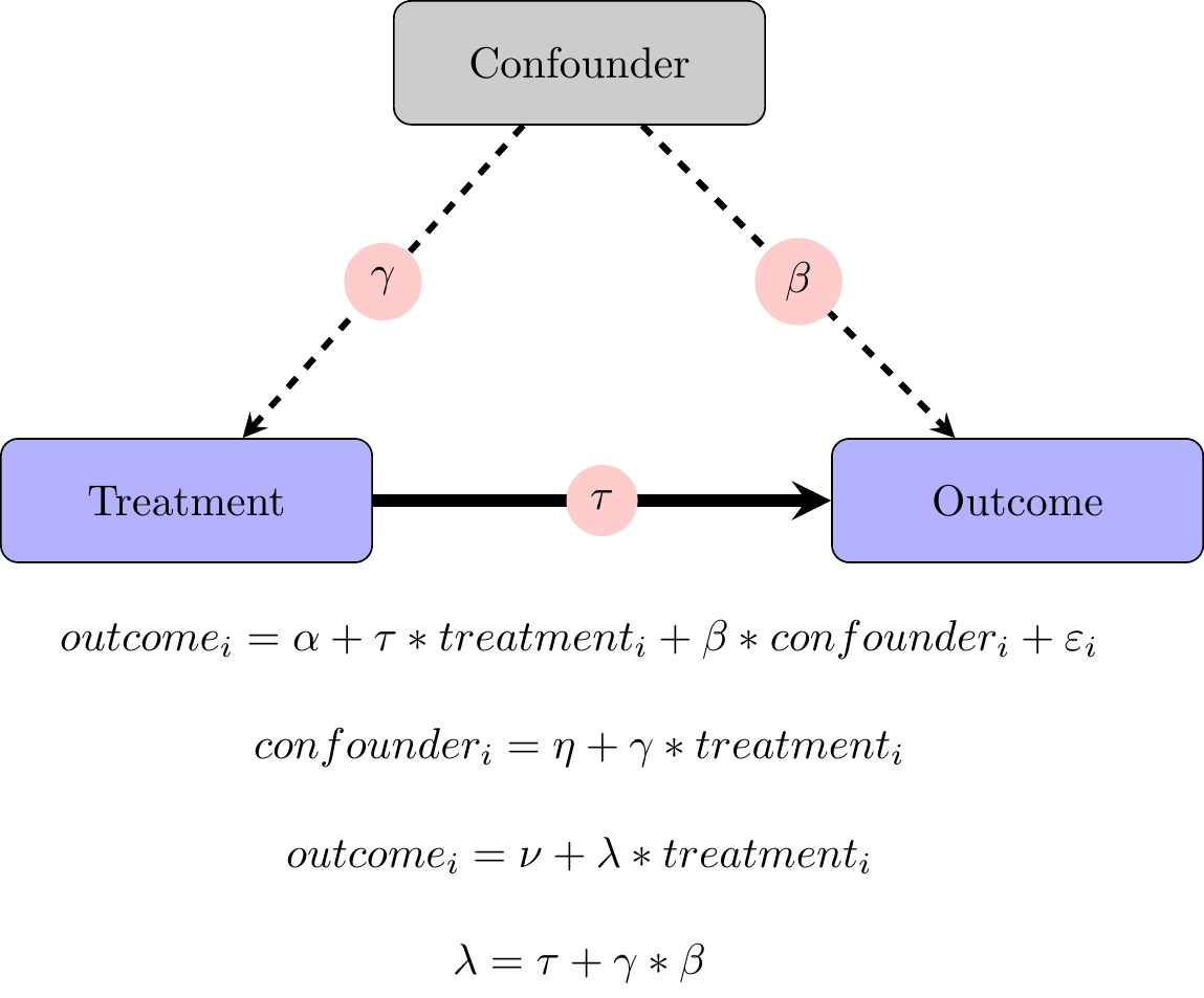
Omitted Variables Bias
Omitted Variables Bias
- True forms of data:
- \(x = 2 + 2*confound + \gamma\)
- \(y = 4 + 5*confound + 2*x + var1 + \varepsilon\)
Omitted Variables Bias
Call:
lm(formula = y ~ x, data = data3)

Residuals:
    Min      1Q  Median      3Q     Max
-57.504 -10.331  -0.022  10.279  59.043

Coefficients:
            Estimate Std. Error  t value Pr(>|t|)
(Intercept) 0.096617   0.319234    0.303    0.762
x           4.486664   0.002678 1675.107   <2e-16 ***
---
Signif. codes:  0 '***' 0.001 '**' 0.01 '*' 0.05 '.' 0.1 ' ' 1

Residual standard error: 15.38 on 9998 degrees of freedom
Multiple R-squared:  0.9964,    Adjusted R-squared:  0.9964
F-statistic: 2.806e+06 on 1 and 9998 DF,  p-value: < 2.2e-16
Omitted Variables Bias
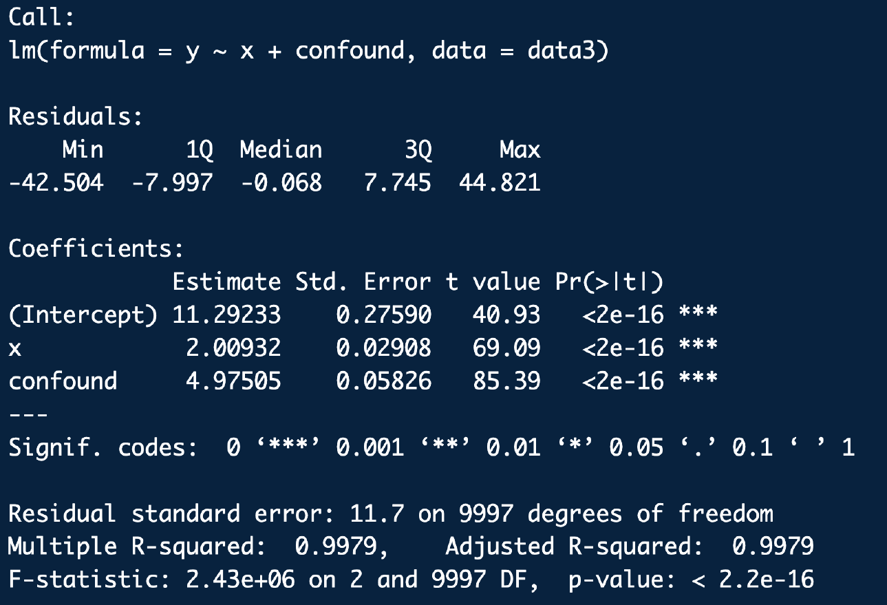
Omitted Variables Bias
Call:
lm(formula = y ~ x + confound, data = data3)

Residuals:
    Min      1Q  Median      3Q     Max
-42.504  -7.997  -0.068   7.745  44.821

Coefficients:
            Estimate Std. Error t value Pr(>|t|)
(Intercept) 11.29233    0.27590   40.93   <2e-16 ***
x            2.00932    0.02908   69.09   <2e-16 ***
confound     4.97505    0.05826   85.39   <2e-16 ***
---
Signif. codes:  0 '***' 0.001 '**' 0.01 '*' 0.05 '.' 0.1 ' ' 1

Residual standard error: 11.7 on 9997 degrees of freedom
Multiple R-squared:  0.9979,    Adjusted R-squared:  0.9979
F-statistic: 2.43e+06 on 2 and 9997 DF,  p-value: < 2.2e-16
Omitted Variables Bias
Omitted Variables Bias
Call:
lm(formula = y ~ x + confound + var1, data = data3)

Residuals:
    Min      1Q  Median      3Q     Max
-21.088  -3.975  -0.028   4.096  23.807

Coefficients:
            Estimate Std. Error t value Pr(>|t|)
(Intercept) 4.181343   0.146864   28.47   <2e-16 ***
x           1.980644   0.014830  133.55   <2e-16 ***
confound    5.036429   0.029710  169.52   <2e-16 ***
var1        1.004484   0.005955  168.68   <2e-16 ***
---
Signif. codes:  0 '***' 0.001 '**' 0.01 '*' 0.05 '.' 0.1 ' ' 1

Residual standard error: 5.965 on 9996 degrees of freedom
Multiple R-squared:  0.9995,    Adjusted R-squared:  0.9995
F-statistic: 6.24e+06 on 3 and 9996 DF,  p-value: < 2.2e-16
Omitted Variables Bias
| mod1 | mod2 | mod3 | |
|---|---|---|---|
| (Intercept) | 0.097 | 11.292*** | 4.181*** |
| (0.319) | (0.276) | (0.147) | |
| x | 4.487*** | 2.009*** | 1.981*** |
| (0.003) | (0.029) | (0.015) | |
| confound | 4.975*** | 5.036*** | |
| (0.058) | (0.030) | ||
| var1 | 1.004*** | ||
| (0.006) | |||
| R2 | 0.996 | 0.998 | 0.999 |
| R2 Adj. | 0.996 | 0.998 | 0.999 |
| + p < 0.1, * p < 0.05, ** p < 0.01, *** p < 0.001 |
Omitted Variables Bias
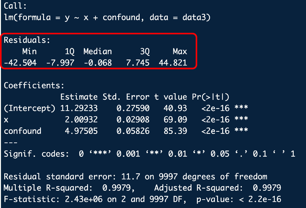
Regression Output
Regression Output
\(y = \alpha + \beta*x + \gamma*confound + \epsilon\)
- Summary statistics for residuals
Regression Output: Intercept Estimate
\(y = \alpha + \beta*x + \gamma*confound + \epsilon\)
- Information about the intercept estimate (\(\alpha\))
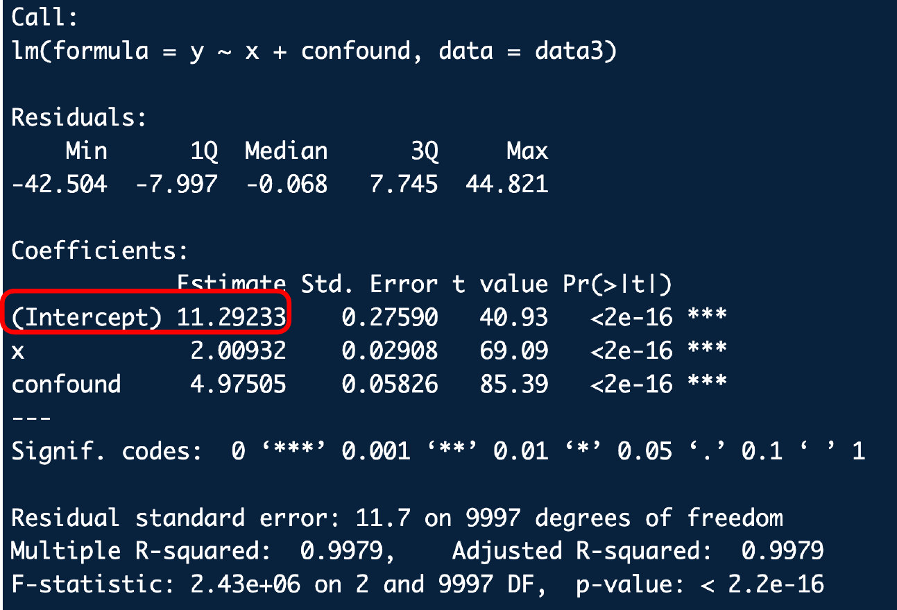
Regression Output: Intercept Estimate
- Tells us the predicted/average value of the outcome when other variables are 0
Regression Output: Coefficient Estimate
\(y = \alpha + \beta*x + \gamma*confound + \epsilon\)
- Information about the coefficient estimate (\(\beta\))
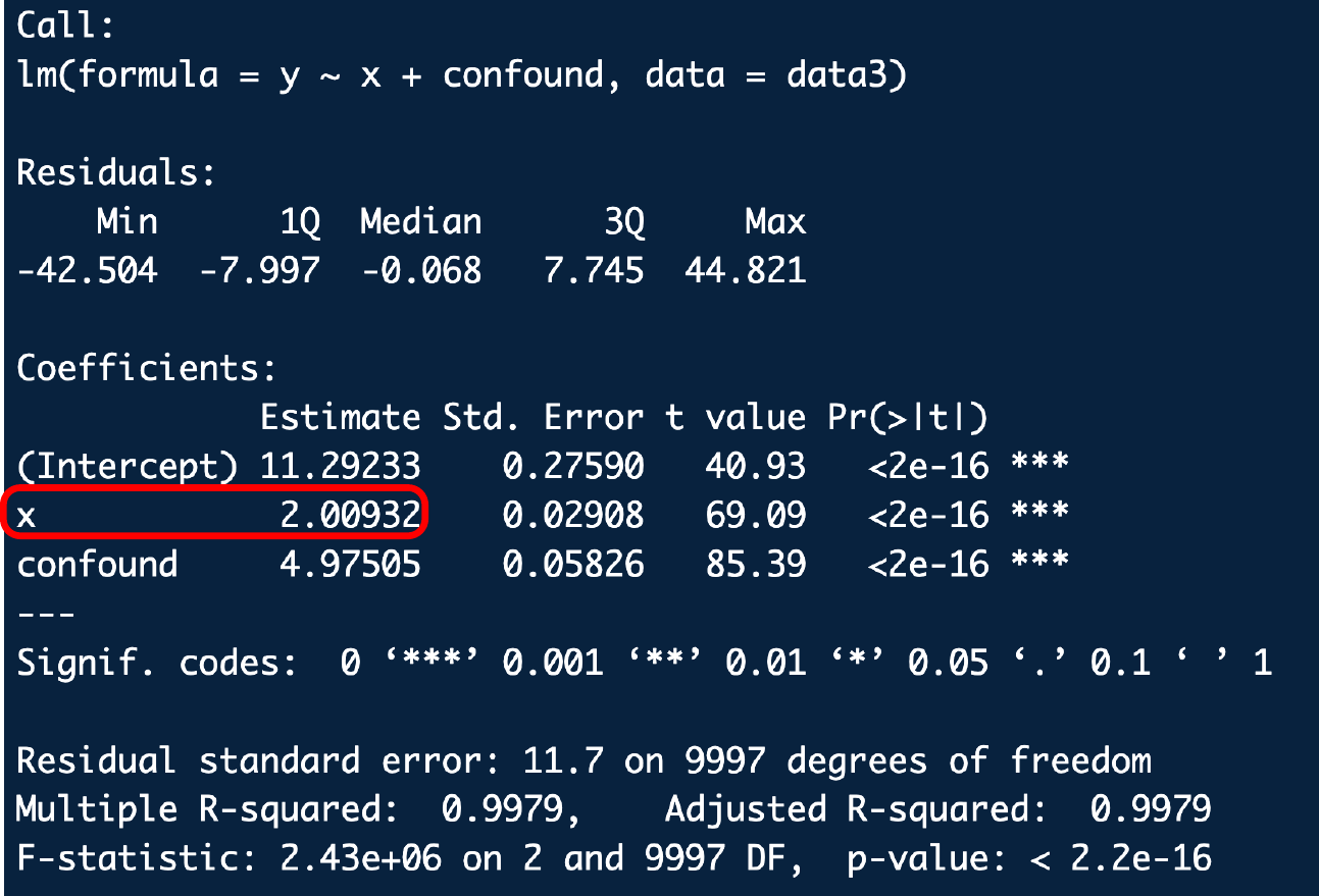
Regression Output: Coefficient Estimate
- Tells us that, holding the other variables in the regression constant,
- We would expect y to be higher by about \(\beta\) when x is higher by one unit
- An increase of 1 in x is associated with a change in the outcome of about \(\beta\)
- The outcome variable is predicted to be higher by about \(\beta\) for each unit increase in the x variable
Regression Output: Hypothesis Testing
- Are the coefficient estimates statistically significant?
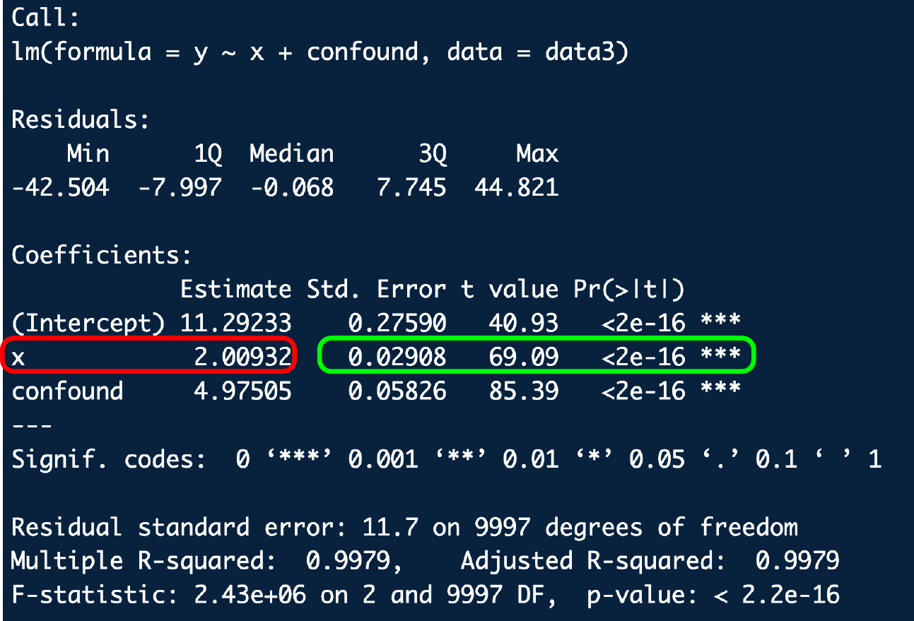
Regression Output: Hypothesis Testing
- Same as standard hypothesis test:
- \(H_0: \beta =0\); \(H_A: \beta \neq 0\)
- \(t\textit{-}statistic=\frac{estimate- 0}{SE}\)
Substantive vs. Statistical Significance
- Statistical Signficance:
- How likely are we to observe the results we observe if the null hypothesis is true?
- Substantive Significance:
- How large or meaningful is our estimate?
Substantive vs. Statistical Significance
- Estimate can be:
- substantively significant without being statistically significant
- statistically significant without being substantively significant
- both
- neither
Tidy Regression Tables
- Can use
modelsummarypackage in R to make nice regression tables
Tidy Regression Tables
| Model 1 | |
|---|---|
| (Intercept) | 0.097 |
| (0.319) | |
| x | 4.487 |
| (0.003) | |
| R2 | 0.996 |
| R2 Adj. | 0.996 |
| Num.Obs. | 10000 |
Linear Regression
