Section 4: Statistical Relationships
2/21/23
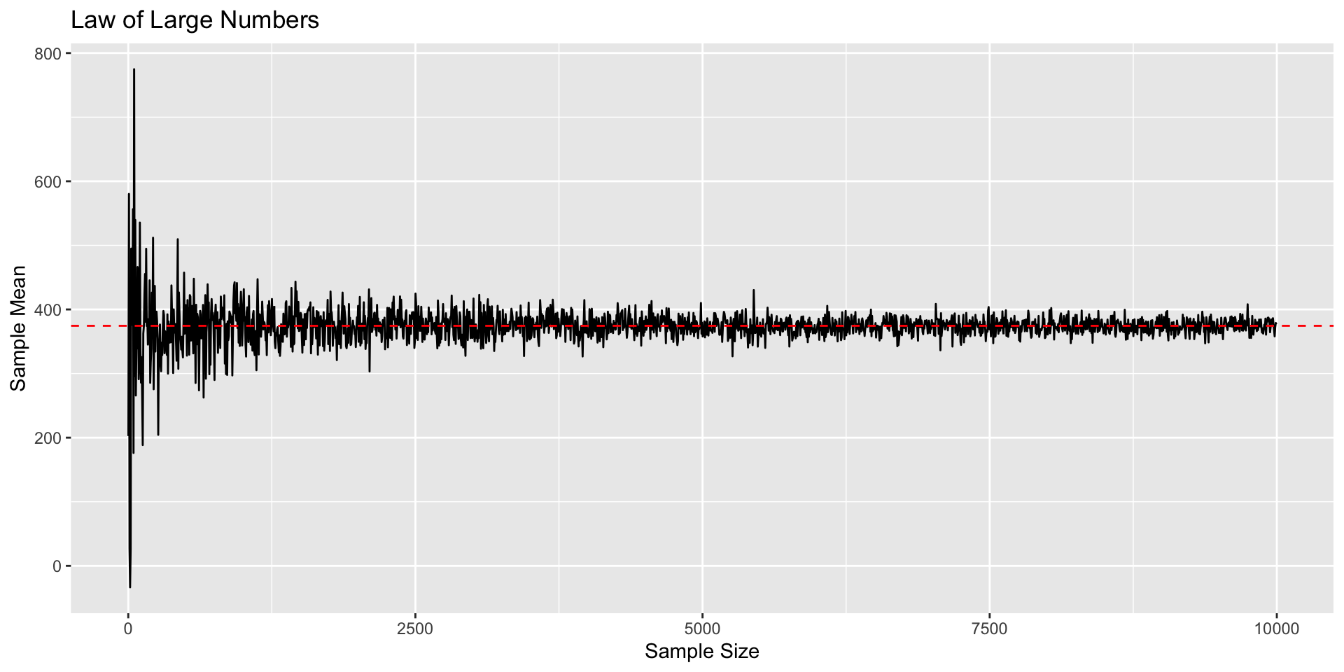
Law of Large Numbers
As \(n \to \infty\), sample mean approaches true population mean:
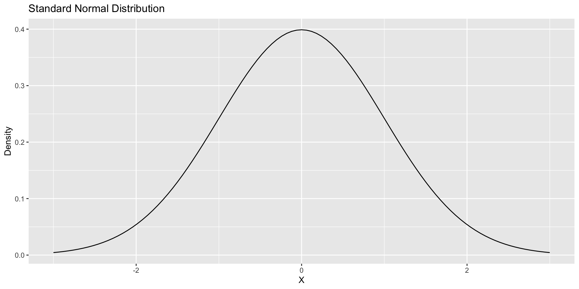
Central Limit Theorem
- What’s more, As \(n \to \infty\), \(\frac{\bar{X}_n - \mu}{\sigma/\sqrt{n}} \to N(0, 1)\)
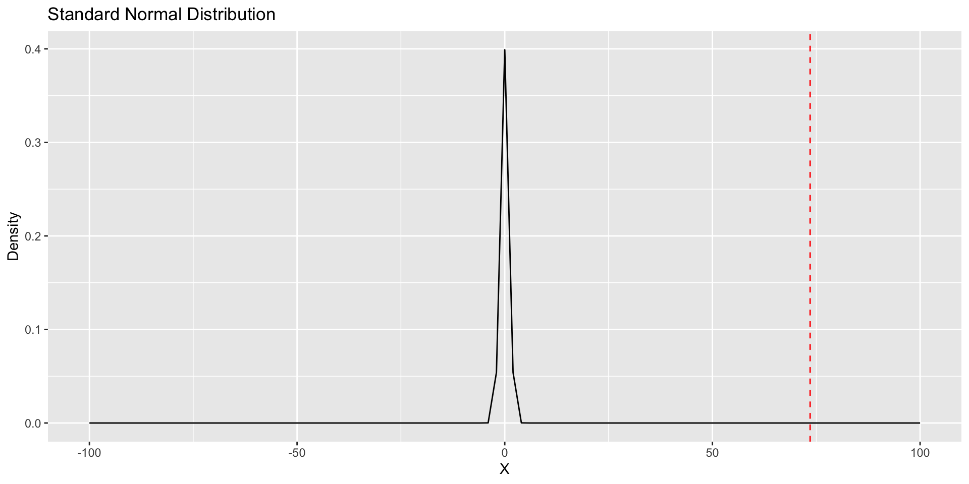
Hypothesis Testing: Example
Hypothesis Testing: Example
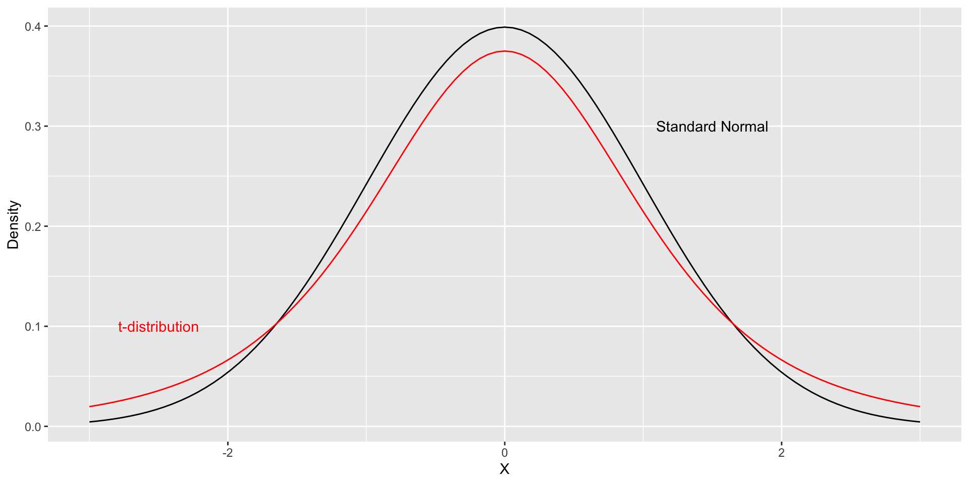
T Distribution
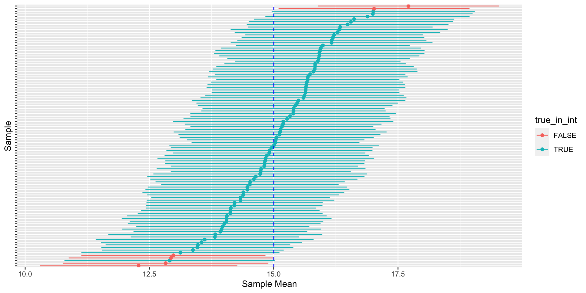
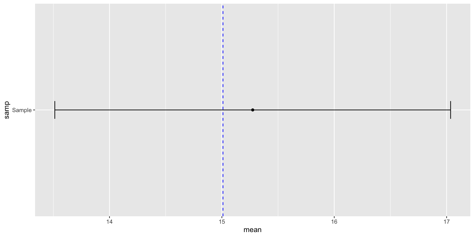
Confidence Intervals: Example
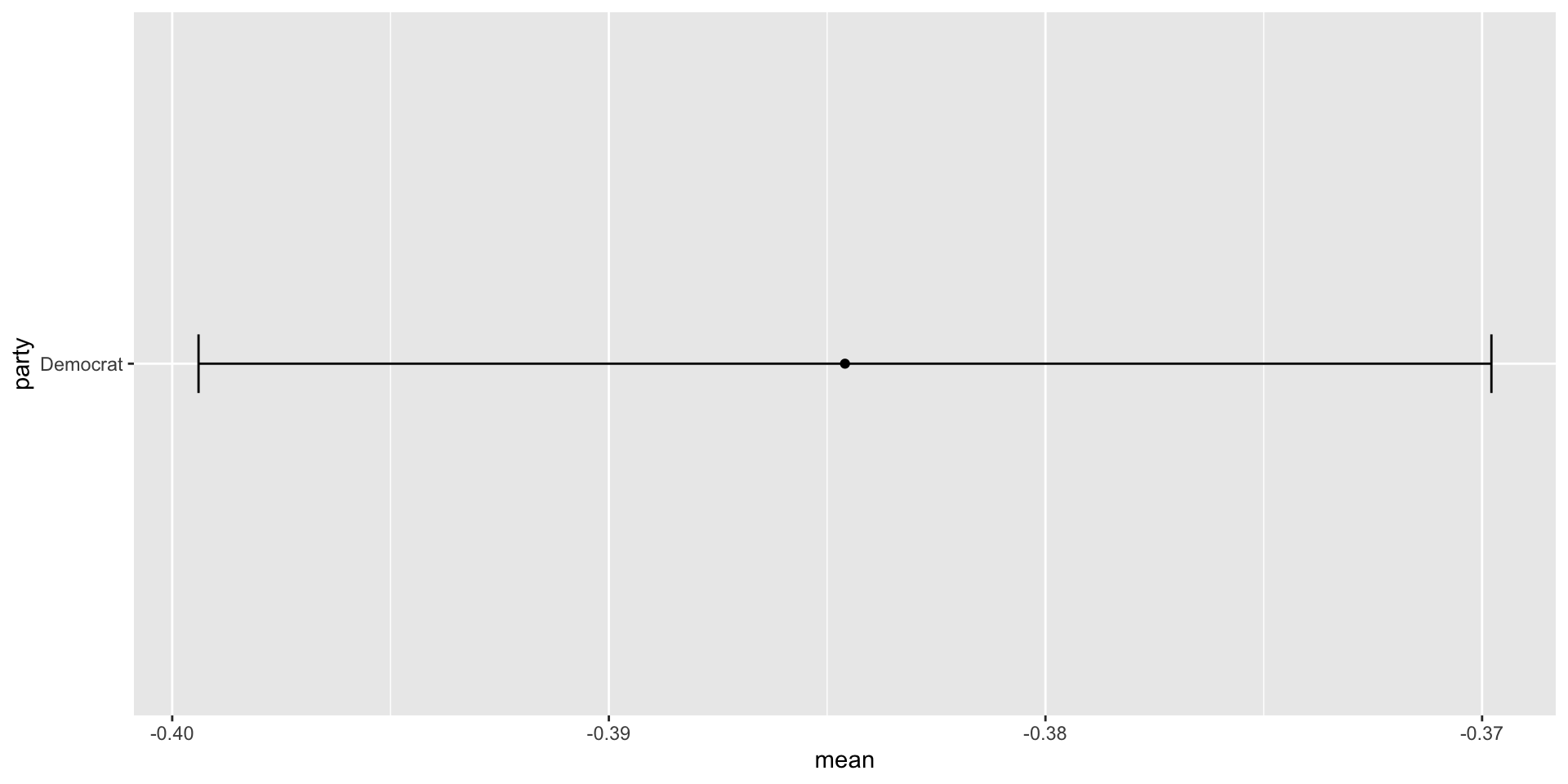
Confidence Intervals: Example
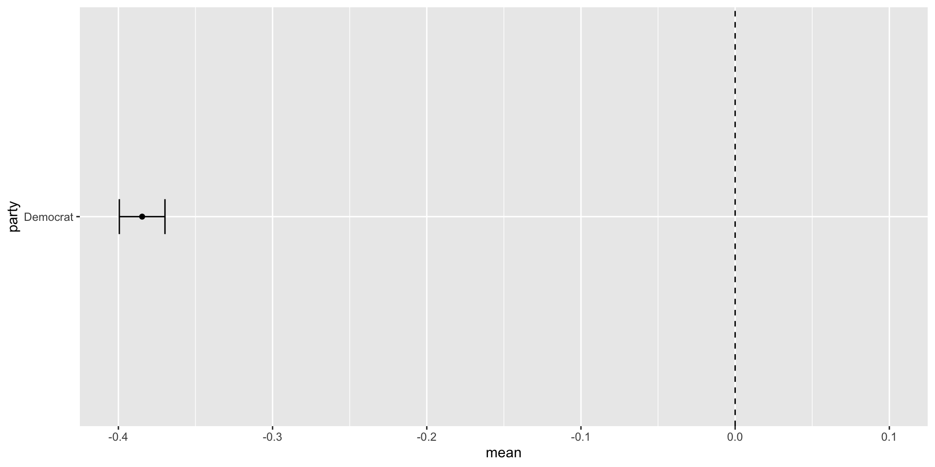
Confidence Intervals
Confidence Intervals