Section 3. Summarizing Data
1/31/23
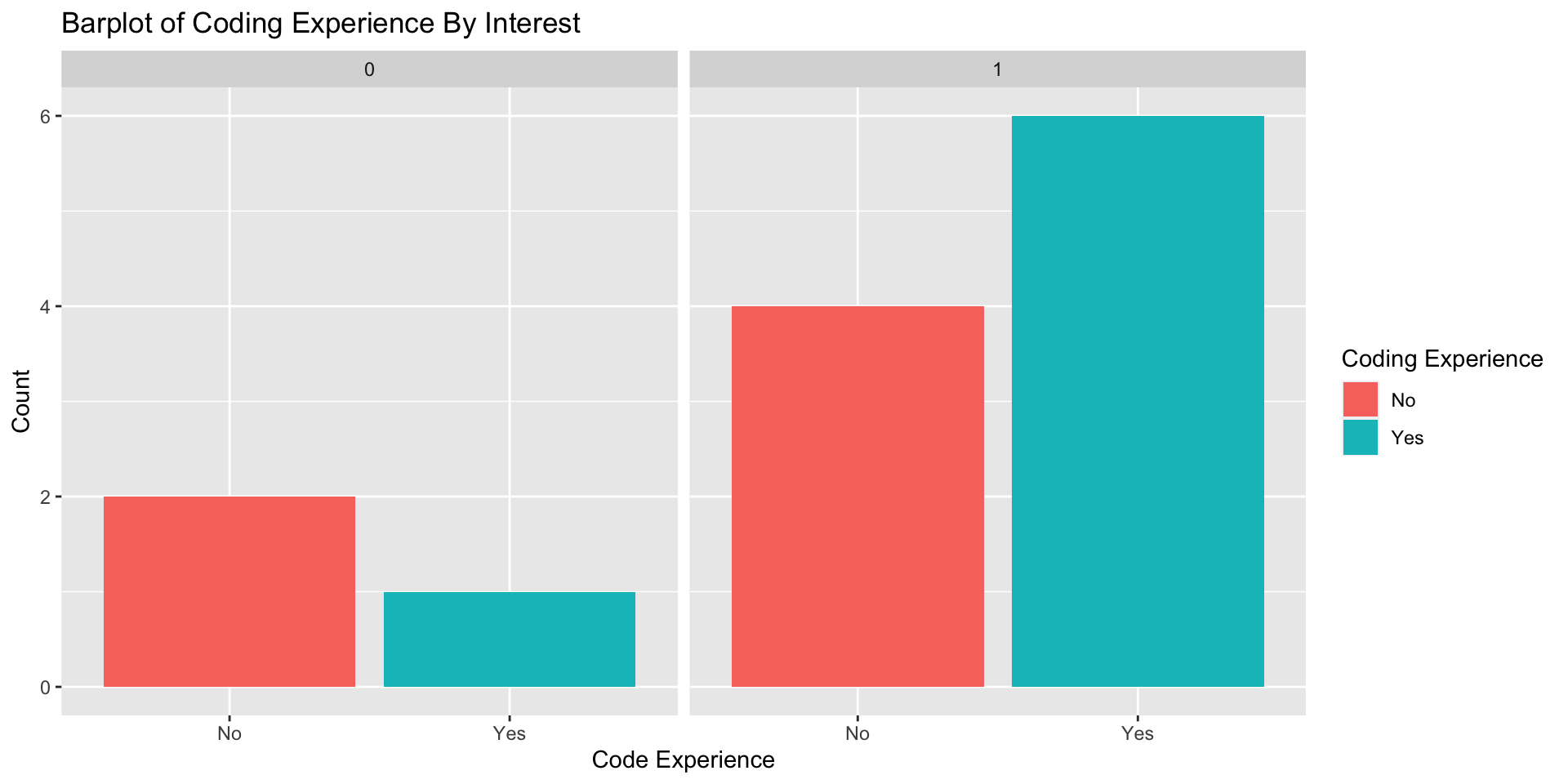
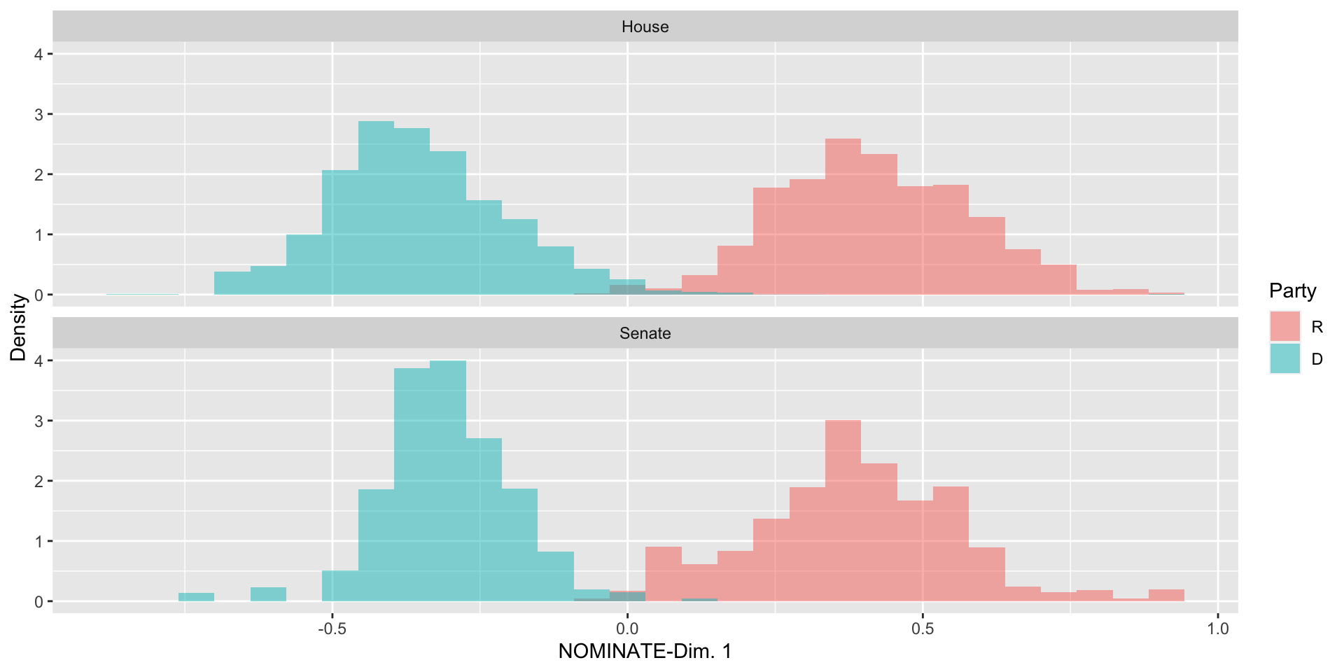
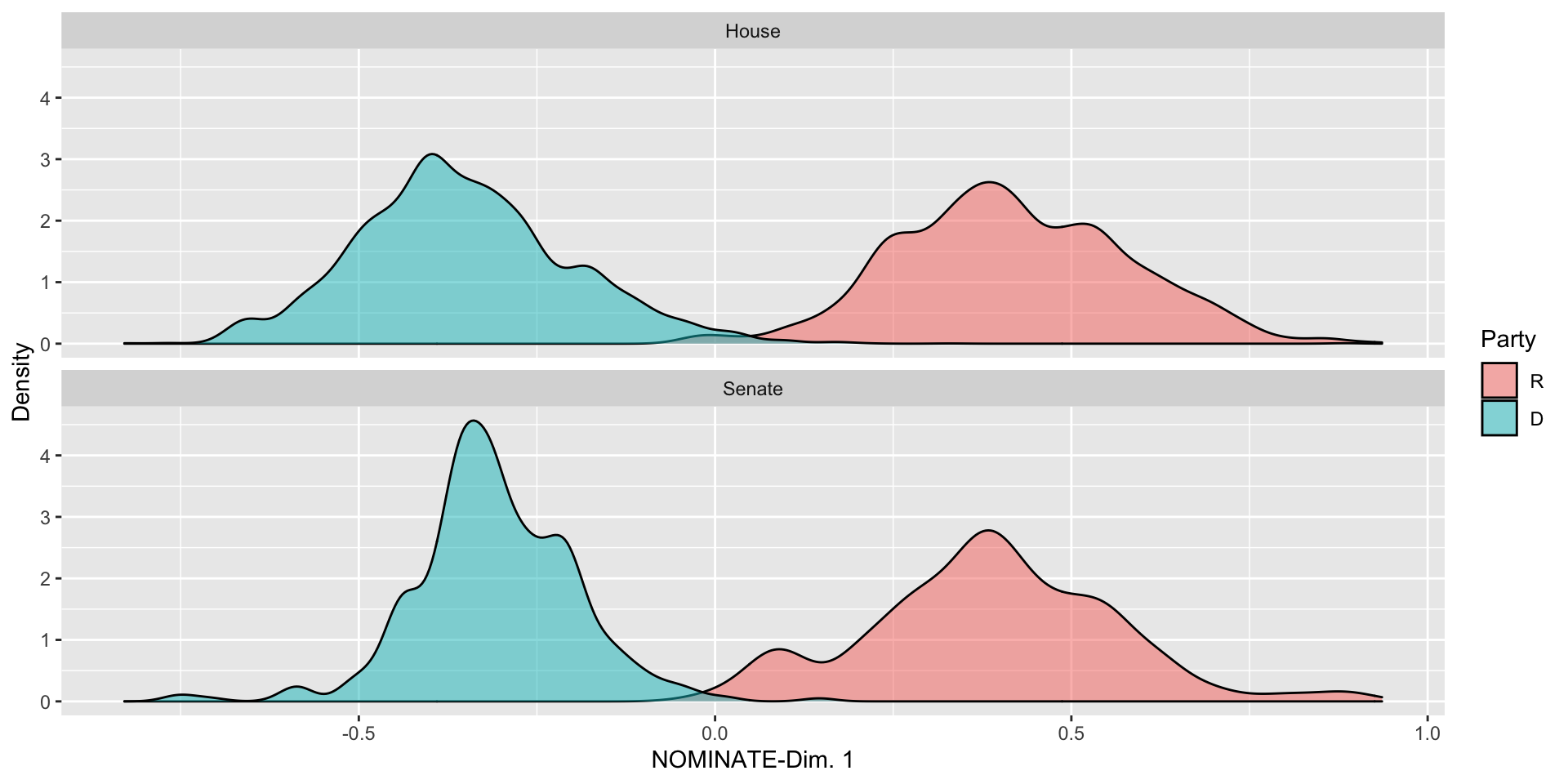
Categorical-Categorical Data: Barplots with Facets
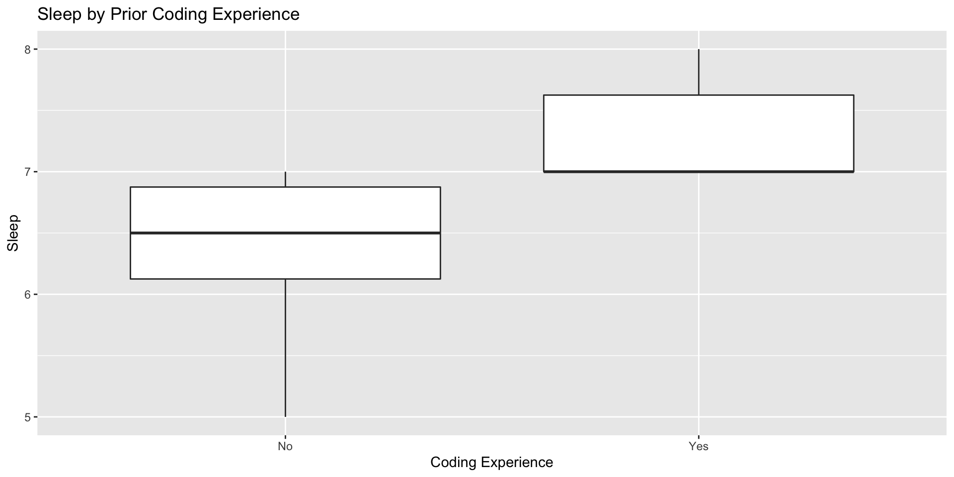
Categorical-Numeric: Box-and-Whisker Plots
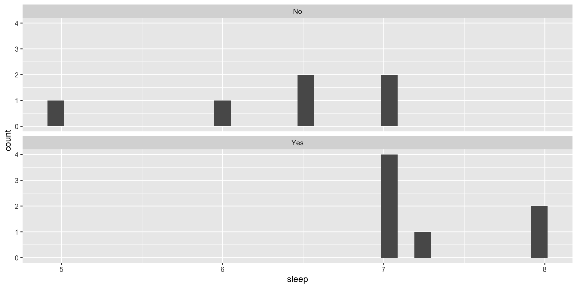
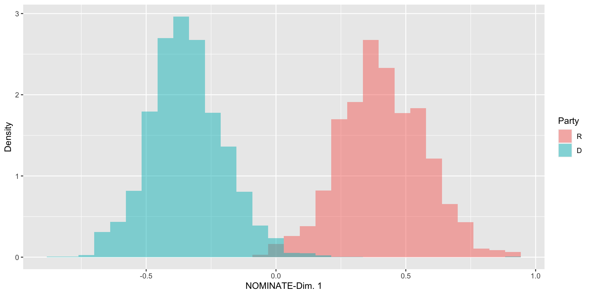
Categorical-Numeric: Histograms
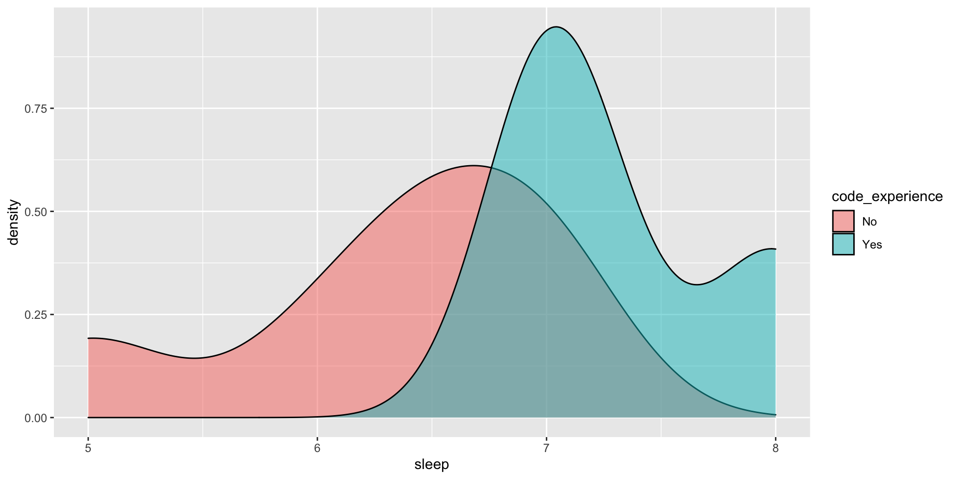
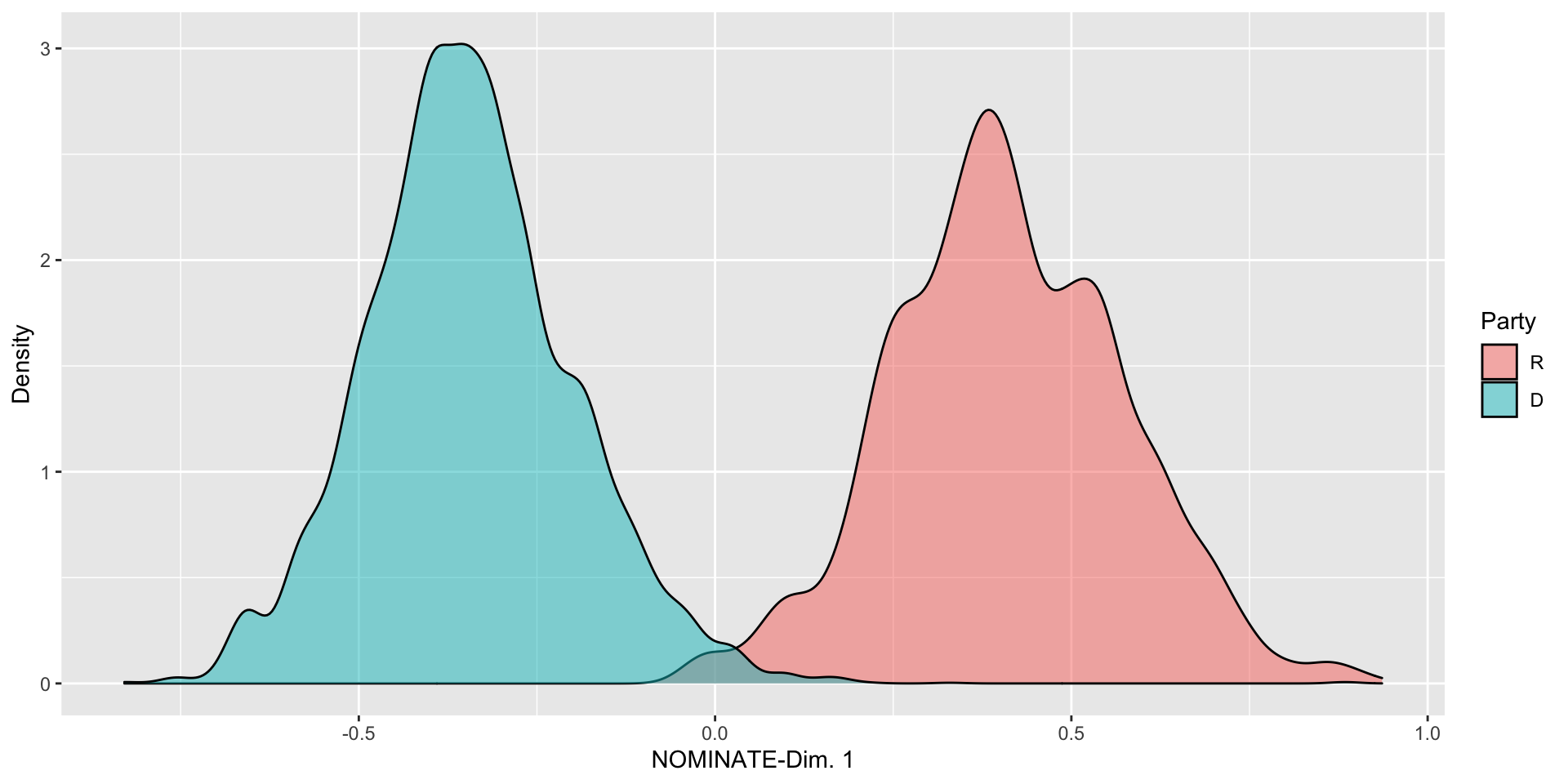
Categorical-Numeric: Density Plots
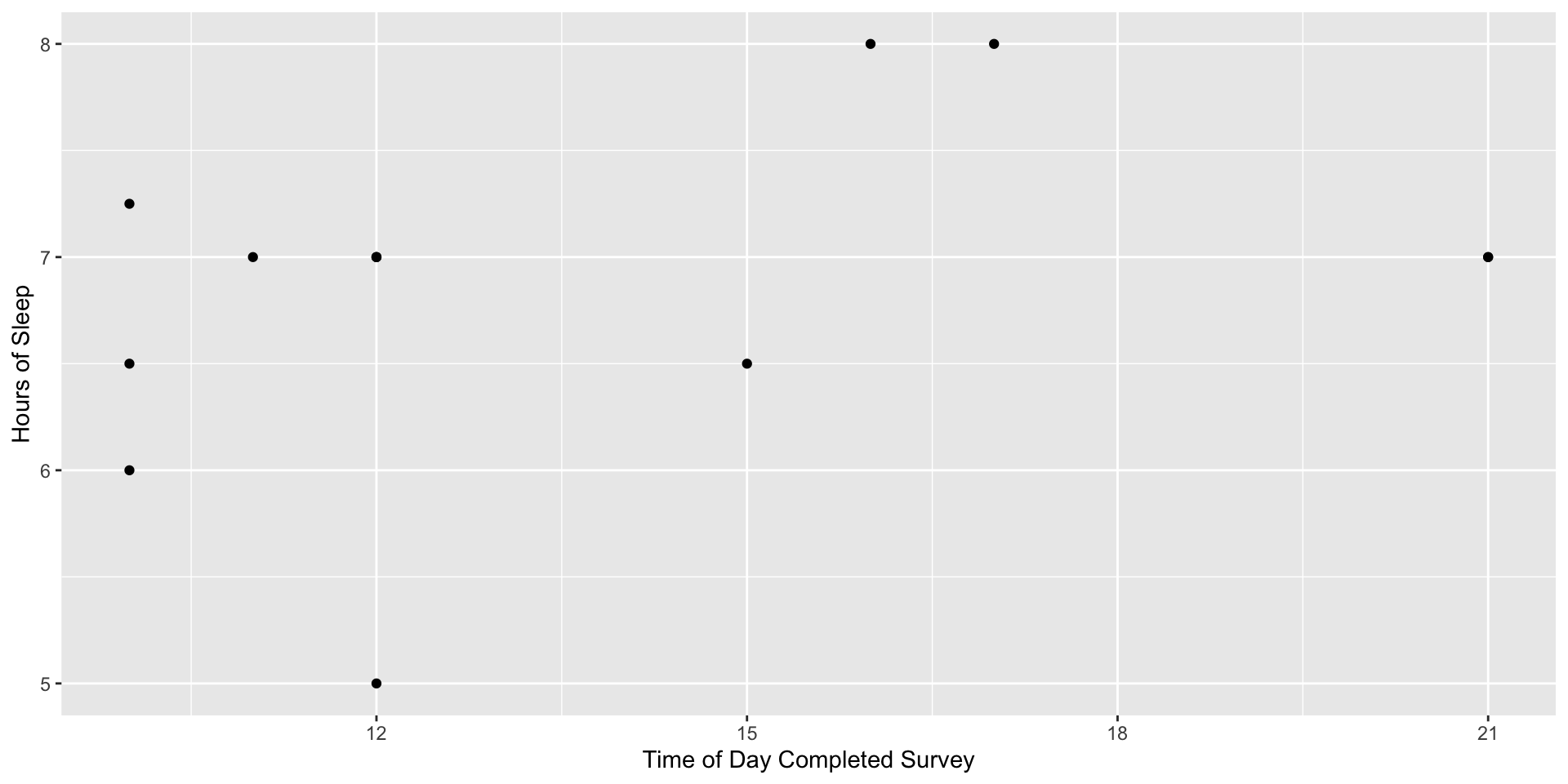
Numeric-Numeric Data: Scatterplots
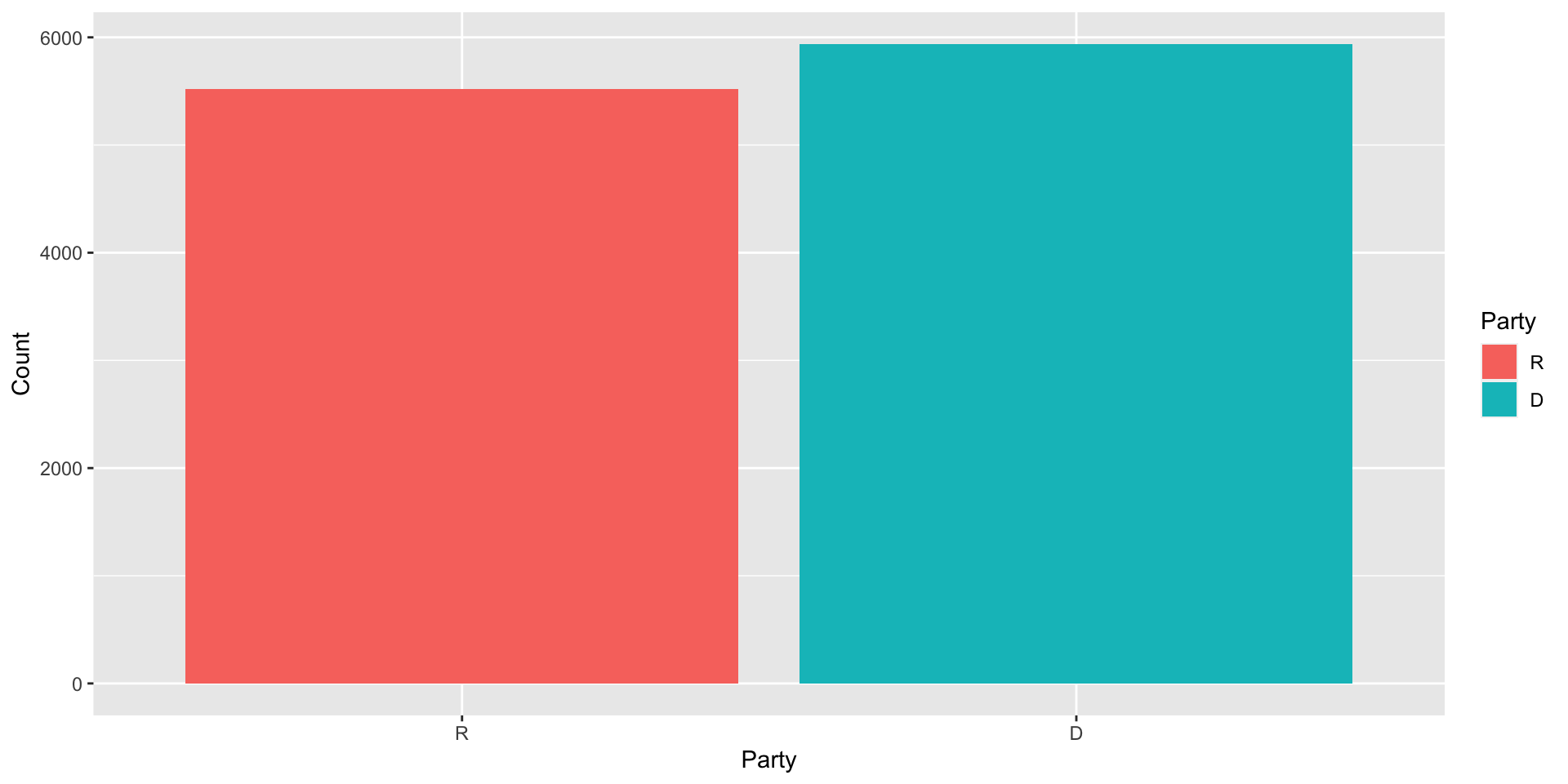
Summarizing Data: Univariate
- Create a barplot of party membership with fill set to party variable
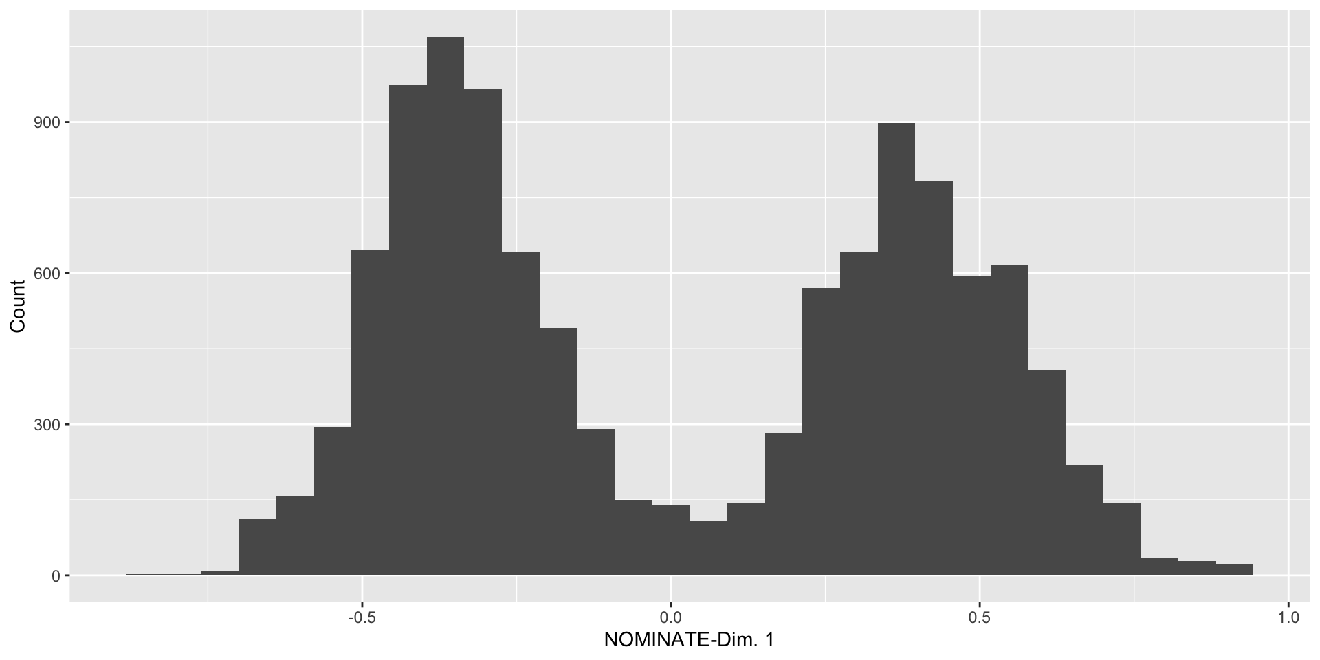
Summarizing Data: Univariate
- Create a histogram of
nominate_dim1- What stands out to you in this histogram?
Summarizing Data: Bivariate and Beyond
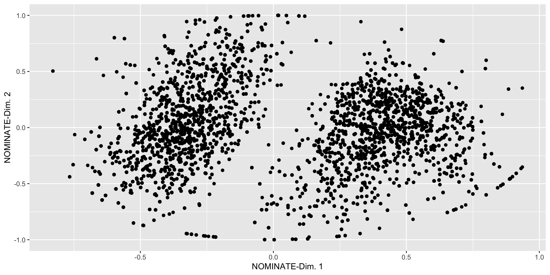
- Numeric-Numeric:
- Create a scatterplot of
nominate_dim2againstnominate_dim1
- Create a scatterplot of
Summarizing Data: Bivariate and Beyond
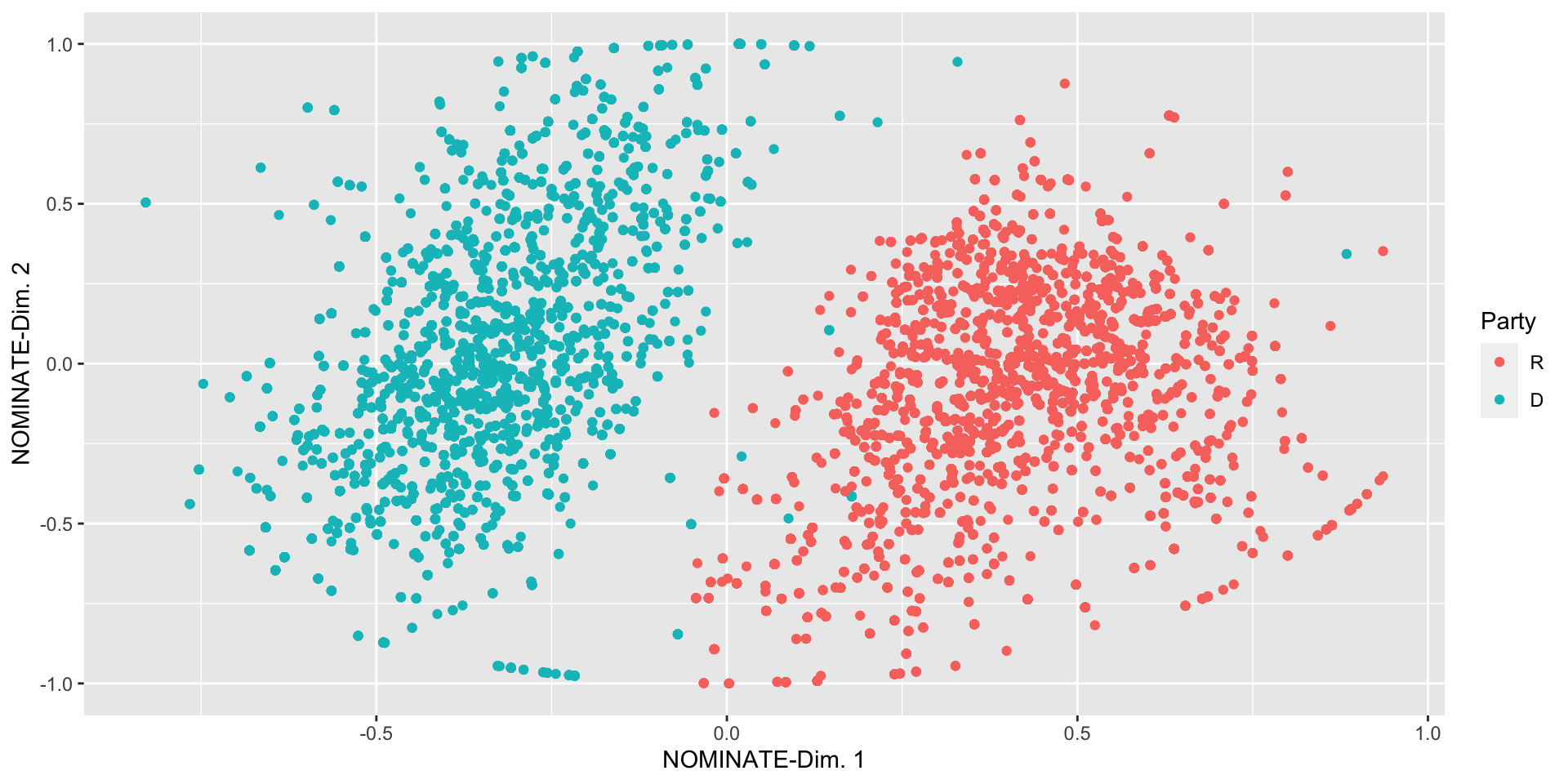
- Numeric-Numeric-Categorical
- Color the above scatterplot by party
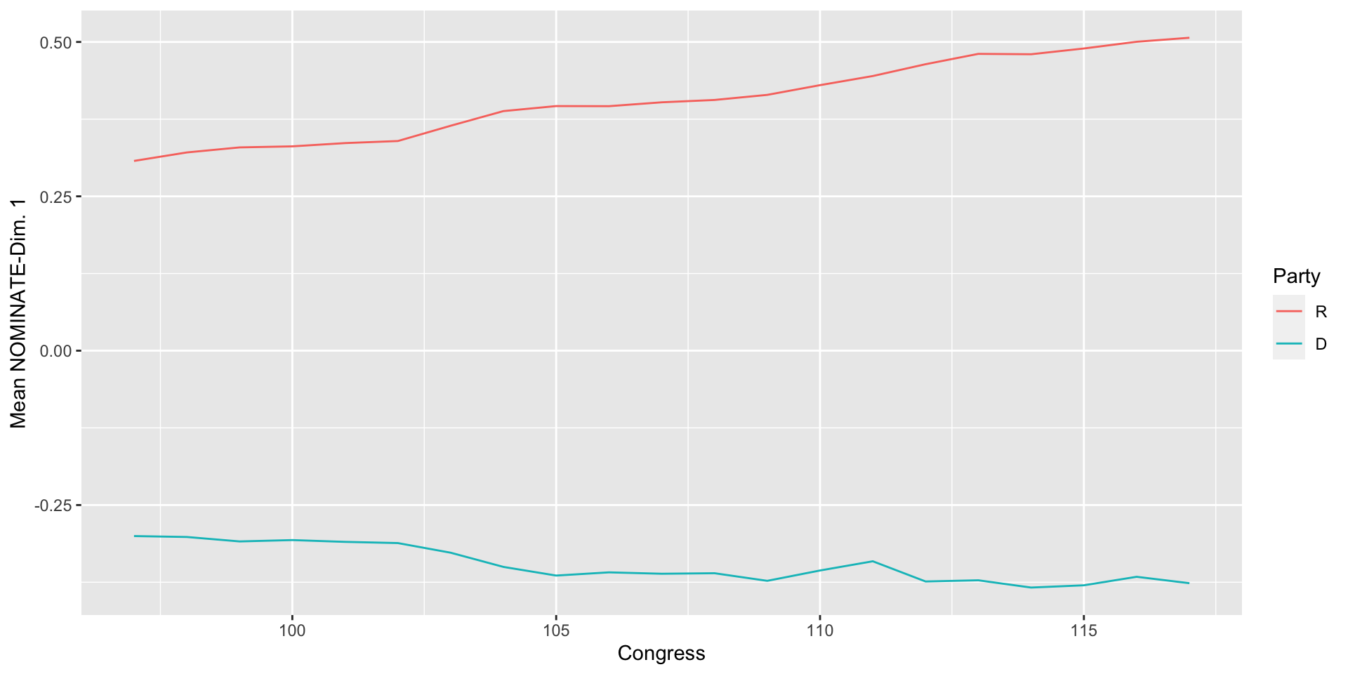
Line Plots
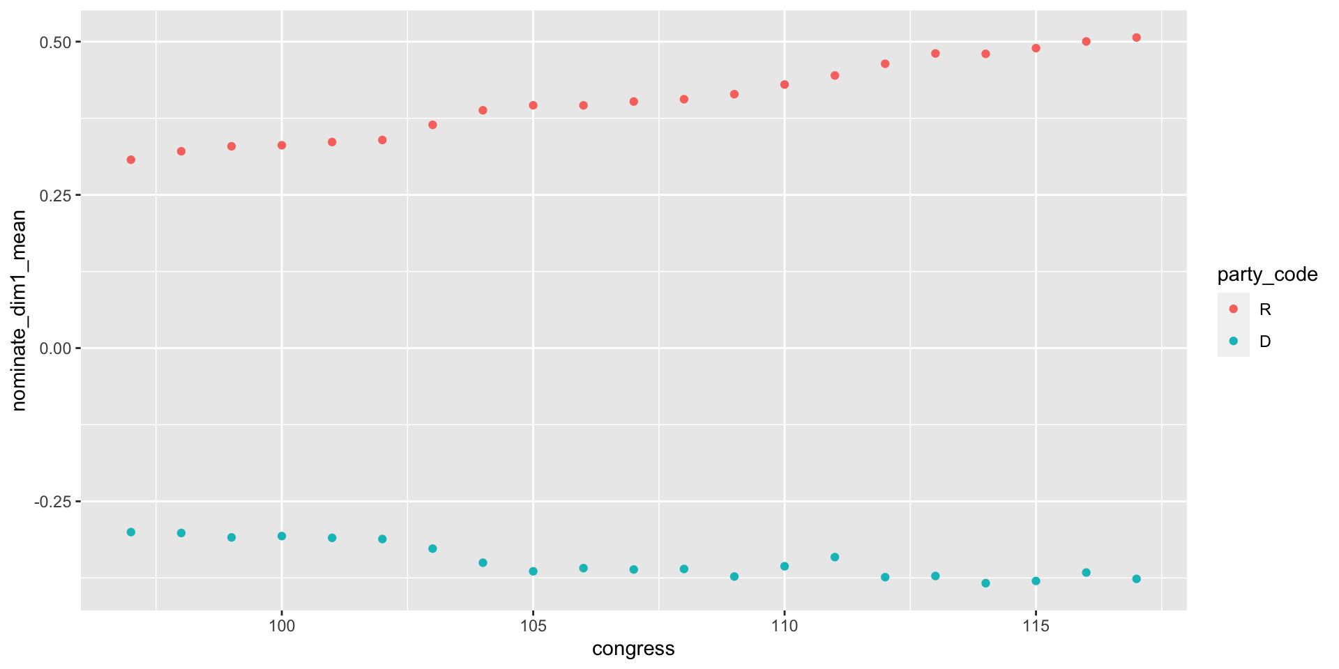
Line Plots
- To make a line plot, we just switch one line of code:
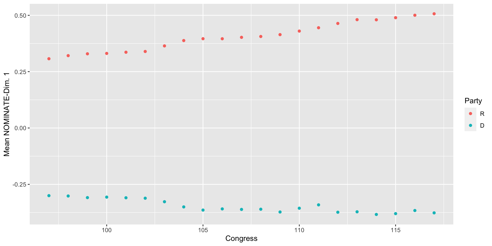
Line Plots
- To make a line plot, we just switch one line of code: