[1] 23.8[1] 23.81/31/23
setwd("/path/to/your/folder")sum(), mean(), min(), max(), sqrt()c()x <- 1:3Types of Objects in R
Summarizing Data in One Variable
Working with Real Data in R
Summarizing Data in One Variable
Working with Real Data in R
Integers int type
Doubles
Ways of Summarizing (Univariate):
summary() functionhist()Ways of Summarizing (Bivariate):
\(Var(x) = \sigma^2 = \frac{1}{n-1}\sum_{i=1}^n(x_i - \bar{x})^2\)
\(sd(x) = \sigma = \sqrt{\frac{1}{n-1}\sum_{i=1}^n(x_i - \bar{x})^2}\)
\(Var(x) = \sigma^2 = \frac{1}{n-1}\sum_{i=1}^n(x_i - \bar{x})^2\)
summary() function
x %>% function()
mutate() to create and change column(s)Data
Plot Foundation: ggplot(data, aes())
+aes(): aesthetic arguments
Character chr data
Factors
Ways of Summarizing (Univariate):
Ways of Summarizing (Bivariate):
factor()factor(variable, levels = c(...), labels = c(...))
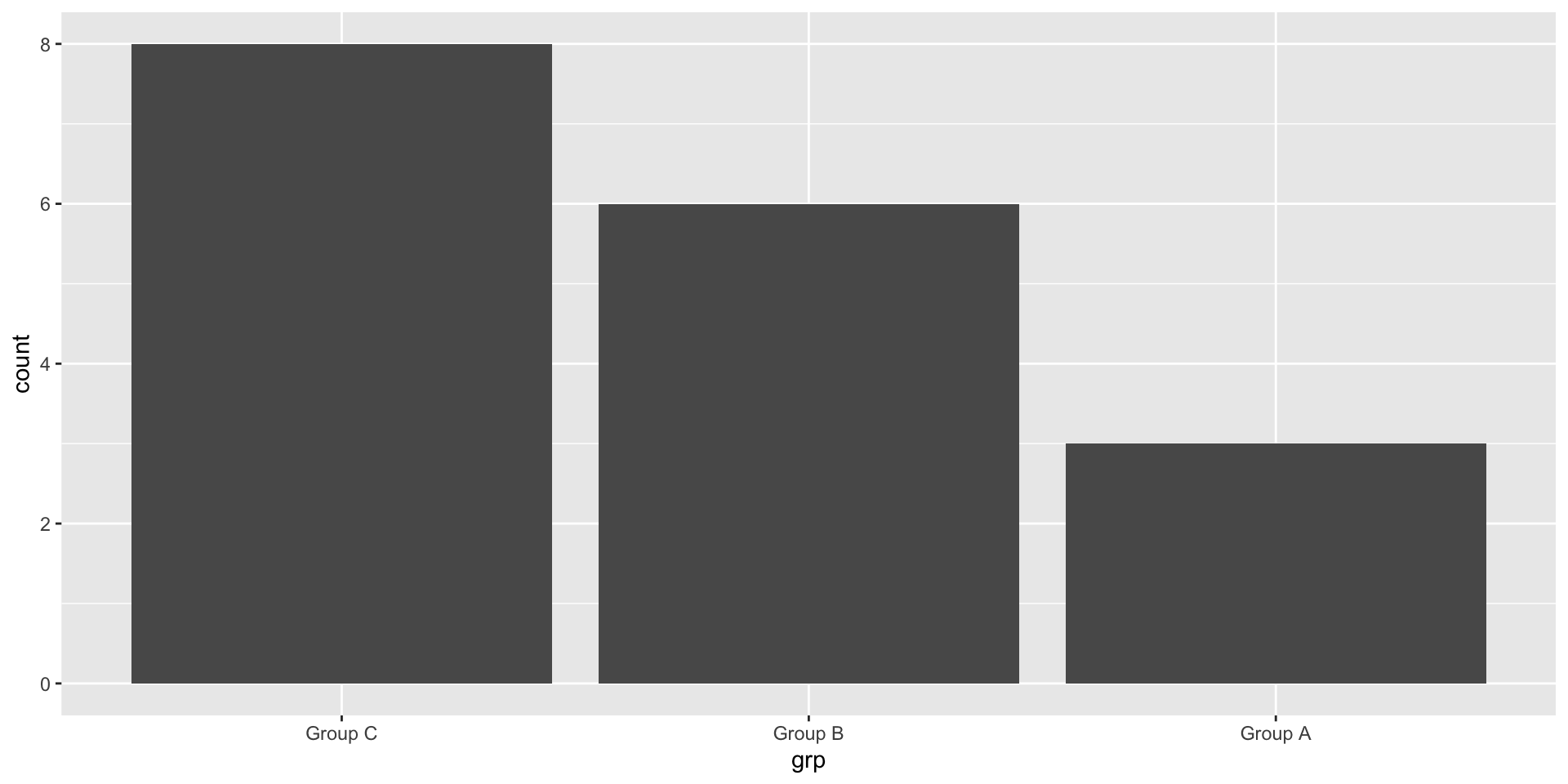
[1] "A" "A" "A" "B" "B" "B" "B" "B" "B" "C" "C" "C" "C" "C" "C" "C" "C"table()
x==y
x<y
x>=y
| Operator | Meaning |
|---|---|
| == | equal to |
| < | less than |
| > | greater than |
| <= | less than or equal to |
| >= | greater than or equal to |
| %in% | in |
[]
[row, column][1] 6# A tibble: 1 × 1
grp
<fct>
1 Group A$
$ as vectorDownload survey responses from Courseworks
Put file into course folder
Set working directory in R or open course RProject
Read file into R using tidyverse:
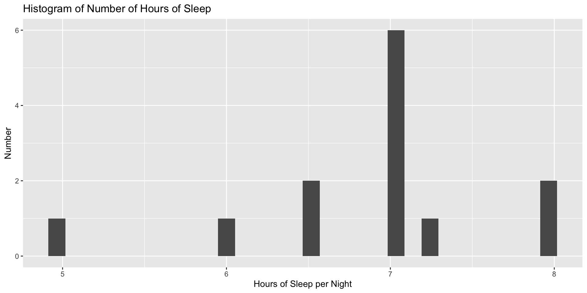
What is the median number of hours of sleep students in this section get each night? How about the standard deviation and range?
See if you can reproduce this plot:
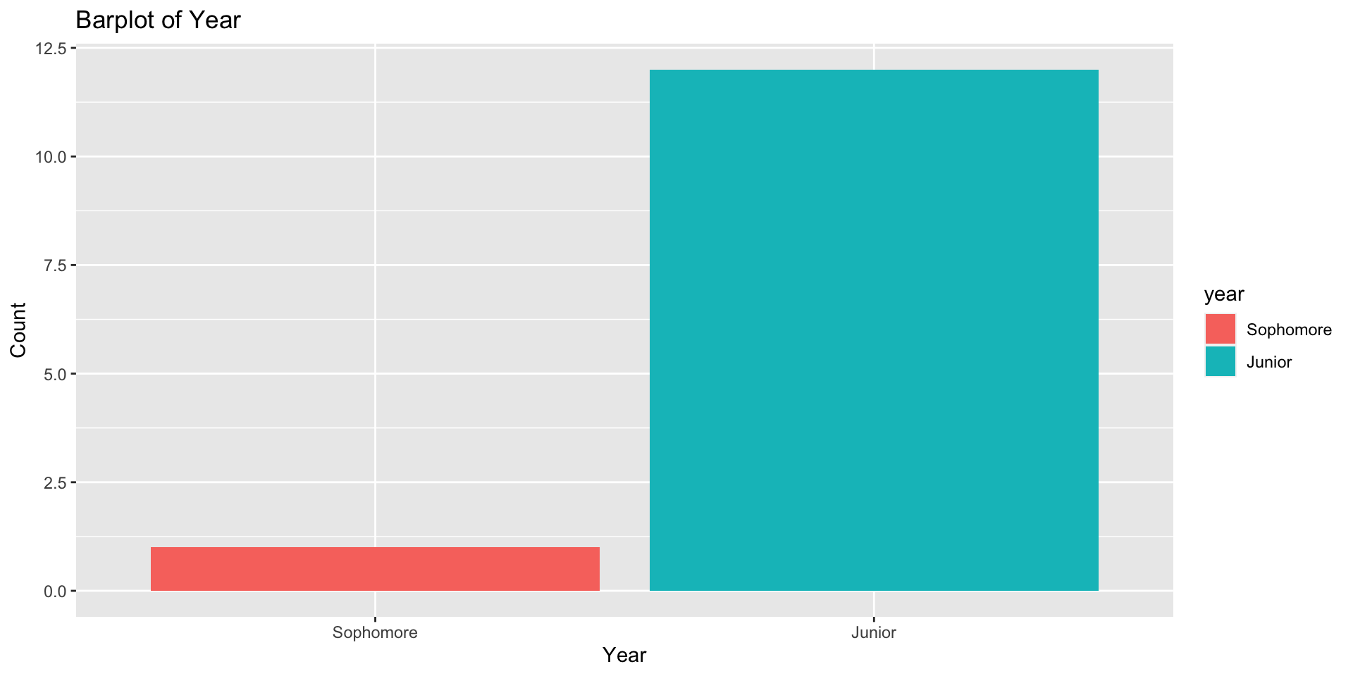
Make the variable year into a factor, and reorder in proper order
mutate() functionMake a proportion table from the new factor variable year
Try making a barplot for the factor variable year with each year in a different color
year into a factor, and reorder in proper orderMake a proportion table from the new factor variable year
Try making a barplot for the factor variable year with each year in a different color
year into a factor, and reorder in proper orderyear
First Year  Sophomore     Junior     Senior
0.00000000 0.07692308 0.92307692 0.00000000 year with each year in a different coloryear with each year in a different colormodelsummary packagemodelsummary packageOften data incomplete or missing altogether
R shows as NA
Some functions will only output missing data if NAs are present
mutate()filter() and logical conditionsggplot(data, aes())+factor(variable, levels = c(...), labels = c(...))na.rm=TRUE argumentSummarizing more than one variable
“If” Statements
For Loops
Introduction to R